Active Learning, part 2: the Practice

This blog post is the continuation of Active Learning, part 1: the Theory, with a focus on how to apply the said theory to an image classification task with PyTorch.

In part 1 we talked about active learning: a semi-supervised machine learning approach in which the model figures out which of the unlabelled data would be most useful to get the labels for. As the model gets access to more (data, label) pairs, its understanding of what training samples are most informative supposedly grows, allowing us to get away with fewer labeled samples without compromising the model's final performance. The hardest part of the process is determining the aforementioned informativeness of the unlabeled samples. The choices are dictated by the selected query strategy, the most common strategies having been discussed in the previous post.

Before we move on to the code, let us remind ourselves of the steps inside the active learning loop:

1. The _oracle (e.g. you) labels some of the data, and adds it to the labeled dataset L.
2. The model gets trained on L.
3. Using a query strategy, the model determines which samples from the unlabelled dataset U it would most like to have labeled next.
4. A request to label the data chosen in step 3 gets sent to the oracle, and we go back to step 1.

There are, of course, many different ways of implementing the steps above. In this blog post, I am going to go through the decisions that I made for my PyTorch implementation, in the hope that it will help you easily adjust my code (see the Jupyter notebook on GitHub) to your situation.

Quickstart for the Docker Crowd

docker run -it -p 8888:8888 --shm-size=16g opetrova/active_dogs
root@6baef783fa64:/workspace# jupyter notebook --port 8888 --allow-root
Copy code

Copy the bottom URL, paste it into your browser, and get training! Both the notebook and the datasets are included.

Poodles & Co.

To demonstrate how active learning works in practice, I chose a ten-breed subset of the Stanford Dogs Dataset for my image classification task. Technically, the project employs both transfer and active learning, as I start with a model that has been pre-trained on the ImageNet. The latter actually includes the ten dog breeds among its classes. This allows me to illustrate quite a few things with a very small number of training samples, since the training mostly comes down to the network figuring out that the ten newly added output nodes correspond to one of: chihuahua, pekinese, basset, whippet, malinois, collie, great dane, chow, and miniature and standard poodles. Ever tried telling miniature and standard poodles apart from a photo? Not an easy task, and I bet that that's the decision boundary that the margin query strategy will focus on. Let us continue to find out!

The Data

Typically, I start my machine learning projects with setting up the data pipeline. In PyTorch, this usually involves writing a custom dataset class that inherits torch.utils.data.Dataset and is then used together with an instance of torch.utils.data.DataLoader to get the data nicely shuffled and split into mini-batches, ready for training. Normally I would write two different dataset classes for unlabelled and labeled data, however, in the case of active learning, the samples will actually go from one category to the other in the course of training. Thus, here we take a different approach: all of the training data belongs to the same dataset. There are two values associated with each sample: 1) a class label (set to an arbitrary value for samples that have not been labeled yet), and 2) a unique index that the various functions that we shall write later on can use to refer to the sample. The dataset object also has a variable called unlabeled_mask: a numpy array with zeros and ones corresponding to labeled and unlabeled samples respectively.

class IndexedDataset(Dataset):

    def __init__(self, dir_path, transform=None, test=False):
        '''
        Args:
        - dir_path (string): path to the directory containing images
        - transform (torchvision.transforms.) (default=None)
        - test (boolean): True for labeled images, False otherwise (default=False)
        '''

        self.dir_path = dir_path
        self.transform = transform

        image_filenames = []
        for (dirpath, dirnames, filenames) in os.walk(dir_path):
            image_filenames += [os.path.join(dirpath, file) for file in filenames if is_image(file)]
        self.image_filenames = image_filenames    

        # We assume that in the beginning, the entire dataset is unlabeled, unless it is flagged as 'test':
        if test:
            # The image's label is given by the first digit of its subdirectory's name
            # E.g. the label for the image file `./dogs/train/6_great_dane/n02109047_22481.webp` is 6
            self.labels = [int(f[len(self.dir_path)+1]) for f in self.image_filenames]
            self.unlabeled_mask = np.zeros(len(self.image_filenames))
        else:
            self.labels =[0]*len(self.image_filenames)
            self.unlabeled_mask = np.ones(len(self.image_filenames))

    def __len__(self):
        return len(self.image_filenames)

    def __getitem__(self, idx):

        img_name = self.image_filenames[idx]
        image = Image.open(img_name)

        if self.transform:
            image = self.transform(image)

        return image, self.labels[idx], idx

    # Display the image [idx] and its filename
    def display(self, idx):
        img_name = self.image_filenames[idx]
        print(img_name)
        img=mpimg.imread(img_name)
        imgplot = plt.imshow(img)
        plt.show()
        return

    # Set the label of image [idx] to 'new_label'
    def update_label(self, idx, new_label):
        self.labels[idx] = new_label
        self.unlabeled_mask[idx] = 0
        return

    # Set the label of image [idx] to that read from its filename
    def label_from_filename(self, idx):
        self.labels[idx] = int(self.image_filenames[idx][len(self.dir_path)+1])
        self.unlabeled_mask[idx] = 0
        return
Copy code

Now let's instantiate ourselves a couple of datasets:

train_dir = './dogs/train'
test_dir = './dogs/test'

train_set = IndexedDataset(train_dir, transform=transforms.Compose([transforms.Resize((224, 224)), transforms.ToTensor()]))

test_set = IndexedDataset(test_dir, transform=transforms.Compose([transforms.Resize((224, 224)), transforms.ToTensor()]), test=True) 

test_loader = DataLoader(test_set, batch_size=1024, shuffle=False, num_workers=10)
Copy code

Notice that so far we have only created the test DataLoader, but not one for training. The reason for this is that we are actually going to create a new training DataLoader each time we update the dataset by labeling some of the data. Luckily, DataLoaders are cheap!

The Model

To keep things simple for the purposes of the tutorial, we'll start with a pre-trained ResNet18 model whose output layer we replace with 10 nodes - for our 10 category classification problem.

# Number of classes in the classification problem
n_classes = 10

# The classifier is a pre-trained ResNet18 with a random top layer dim = n_classes
classifier = models.resnet18(pretrained=True)
num_ftrs = classifier.fc.in_features
classifier.fc = nn.Linear(num_ftrs, n_classes)
classifier = classifier.to(device) 

criterion = nn.CrossEntropyLoss()
optimizer = optim.SGD(classifier.parameters(), lr=0.01, momentum=0.9, dampening=0, weight_decay=0.0001)     
Copy code

Normally we would have some amount of labeled data to start with, and pre-train the model on those samples before we get into active learning. Otherwise, we can go ahead and query the oracle for, say, twenty random samples' labels:

# Label the initial subset
query_the_oracle(classifier, device, train_set, query_size=20, interactive=False, query_strategy='random', pool_size=0)
Copy code

Now let us look at the query process in a little more detail:

Querying the Oracle

In the previous section, we called query_the_oracle() to annotate 20 unlabelled samples, chosen at random from the train_set. The interactive argument can be set to True or False depending on whether we want the user to enter the image's label when prompted for it, or if the label is to be read from the image's file name. The reason why the classifier model is passed as one of the function arguments is that any query_strategy (more on them shortly), other than the random one, would need access to the model that we are trying to train.

def query_the_oracle(model, device, dataset, query_size=10, query_strategy='random', 
                     interactive=True, pool_size=0, batch_size=128, num_workers=4):

    unlabeled_idx = np.nonzero(dataset.unlabeled_mask)[0]

    # Select a pool of samples to query from
    if pool_size > 0:    
        pool_idx = random.sample(range(1, len(unlabeled_idx)), pool_size)
        pool_loader = DataLoader(dataset, batch_size=batch_size, num_workers=num_workers,
                                              sampler=SubsetRandomSampler(unlabeled_idx[pool_idx]))
    else:
        pool_loader = DataLoader(dataset, batch_size=batch_size, num_workers=num_workers,
                                              sampler=SubsetRandomSampler(unlabeled_idx))

    if query_strategy == 'margin':
        sample_idx = margin_query(model, device, pool_loader, query_size)
    elif query_strategy == 'least_confidence':
        sample_idx = least_confidence_query(model, device, pool_loader, query_size)
    else:
        sample_idx = random_query(pool_loader, query_size)

    # Query the samples, one at a time
    for sample in sample_idx:

        if interactive:
            dataset.display(sample)
            print("What is the class of this image?")
            new_label = int(input())
            dataset.update_label(sample, new_label)

        else:
            dataset.label_from_filename(sample)
Copy code

A few words on the Pool size in Pool-based Active Learning

In the code above, what is this pool all about? What we are looking at here is pool-based sampling. We select what we believe are the most informative samples out of a pool of unlabeled data. The notion of a pool can be extended to the entire unlabeled dataset that we have, but it does not have to be. In fact, there are several scenarios where it should not, namely:

1. If your data contains outliers that are likely to be picked up by the query strategy that you are using (e.g. the least confidence strategy is often guilty of this). Let's say you have 10 of these in your dataset, and you are querying 20 samples at a time. If your pool is the entire dataset, half of your query will be at best useless (or worse, hurt your model's performance!). If your pool size is 10% of the dataset, however, it will on average contain a single outlier, leaving you with 19 informative samples to label and learn from for the next iteration.
2. If your unlabeled dataset is very large. If you have a huge amount of unlabeled data, it may not make sense to go through all of it every time you look for good samples to label. Take a large chunk of data and select your samples from it instead.

Query Strategies

I have implemented three query strategies: the random one, and two ways to do uncertainty sampling: least confidence and margin. Uncertainty sampling is not without issues, as we discussed in the previous blog post, so one of our goals today is to see whether there is in fact any benefit to using it over simply sampling data at random. The three functions below go through a DataLoader corresponding to the pool of unlabeled data that we are considering, and return a list of indices for the samples from it that should be labeled next.

'''
Each query strategy below returns a list of len=query_size with indices of 
samples that are to be queried.

Arguments:
- model (torch.nn.Module): not needed for `random_query`
- device (torch.device): not needed for `random_query`
- dataloader (torch.utils.data.DataLoader)
- query_size (int): number of samples to be queried for labels (default=10)

'''
def random_query(data_loader, query_size=10):

    sample_idx = []

    # Because the data has already been shuffled inside the data loader,
    # we can simply return the `query_size` first samples from it
    for batch in data_loader:

        _, _, idx = batch
        sample_idx.extend(idx.tolist())

        if len(sample_idx) >= query_size:
            break

    return sample_idx[0:query_size]

def least_confidence_query(model, device, data_loader, query_size=10):

    confidences = []
    indices = []

    model.eval()

    with torch.no_grad():
        for batch in data_loader:

            data, _, idx = batch
            logits = model(data.to(device))
            probabilities = F.softmax(logits, dim=1)

            # Keep only the top class confidence for each sample
            most_probable = torch.max(probabilities, dim=1)[0]
            confidences.extend(most_probable.cpu().tolist())
            indices.extend(idx.tolist())

    conf = np.asarray(confidences)
    ind = np.asarray(indices)
    sorted_pool = np.argsort(conf)
    # Return the indices corresponding to the lowest `query_size` confidences
    return ind[sorted_pool][0:query_size]

def margin_query(model, device, data_loader, query_size=10):

    margins = []
    indices = []

    model.eval()

    with torch.no_grad():
        for batch in data_loader:

            data, _, idx = batch
            logits = model(data.to(device))
            probabilities = F.softmax(logits, dim=1)

            # Select the top two class confidences for each sample
            toptwo = torch.topk(probabilities, 2, dim=1)[0]

            # Compute the margins = differences between the two top confidences
            differences = toptwo[:,0]-toptwo[:,1]
            margins.extend(torch.abs(differences).cpu().tolist())
            indices.extend(idx.tolist())

    margin = np.asarray(margins)
    index = np.asarray(indices)
    sorted_pool = np.argsort(margin)
    # Return the indices corresponding to the lowest `query_size` margins
    return index[sorted_pool][0:query_size]
Copy code

Now that we have labeled some initial images, it is time to pre-train our model on them. How long should we train for? It is up to you to provide a stopping criteria, but best keep it simple since we are going to have to use it every time we process a new group of labeled samples. You could, for instance, train for a set number of epochs, or until the training loss hits a certain threshold value, or while the accuracy of the model on the test set keeps increasing. I chose the latter:

def train(model, device, train_loader, optimizer, criterion):

    model.train()

    epoch_loss = 0

    m_train = 0

    for batch in train_loader:

        data, target, _ = batch
        m_train += data.size(0)
        data, target = data.to(device), target.to(device)

        optimizer.zero_grad()
        output = model(data)
        loss = criterion(output.squeeze(), target.squeeze())
        loss.backward()
        optimizer.step()
        epoch_loss += loss.item()

    return epoch_loss / m_train

def test(model, device, test_loader, criterion, display=False):

    model.eval()

    test_loss = 0
    n_correct = 0

    one = torch.ones(1, 1).to(device)
    zero = torch.zeros(1, 1).to(device)

    with torch.no_grad():
        for batch in test_loader:

            data, target, _ = batch
            data, target = data.to(device), target.to(device)
            output = model(data)
            test_loss += criterion(output.squeeze(), target.squeeze()).item()  # sum up batch loss
            prediction = output.argmax(dim=1, keepdim=True)
            torch.where(output.squeeze()<0.5, zero, one)  # get the index of the max log-probability
            n_correct += prediction.eq(target.view_as(prediction)).sum().item()

    test_loss /= len(test_loader.dataset) 
    if display:
        print('Accuracy on the test set: ', (100. * n_correct / len(test_loader.dataset)))
    return test_loss, (100. * n_correct / len(test_loader.dataset))

previous_test_acc = 0
current_test_acc = 1

while current_test_acc > previous_test_acc:
    previous_test_acc = current_test_acc
    train_loss = train(classifier, device, labeled_loader, optimizer, criterion)
    _, current_test_acc = test(classifier, device, test_loader, criterion)
Copy code

The Active Learning Loop

Active learning is an iterative process that involves going through the four steps outlined in the Introduction until we are satisfied with the model's performance on the validation / test set (or until we run out of our labeling budget, whichever comes first). Let us see what happens when we get our active learning process up and running:

for query in range(num_queries):

    # Query the oracle for more labels
    query_the_oracle(classifier, device, train_set, query_size=5, query_strategy='margin', interactive=True, pool_size=10)

    # Train the model on the data that has been labeled so far:
    labeled_idx = np.where(train_set.unlabeled_mask == 0)[0]
    labeled_loader = DataLoader(train_set, batch_size=batch_size, num_workers=10, sampler=SubsetRandomSampler(labeled_idx))

    previous_test_acc = 0
    current_test_acc = 1
    while current_test_acc > previous_test_acc:
        previous_test_acc = current_test_acc
        train_loss = train(classifier, device, labeled_loader, optimizer, criterion)
        _, current_test_acc = test(classifier, device, test_loader, criterion)


    # Test the model:
    test(classifier, device, test_loader, criterion)
Copy code

During each iteration, you get prompted to label a few images, which are then added to the labeled training set. At this point, the training of the classifier resumes: it gets trained on all the labeled samples that you have gathered so far. Here is what that process may look like from the user's (I mean, the oracle's) perspective:

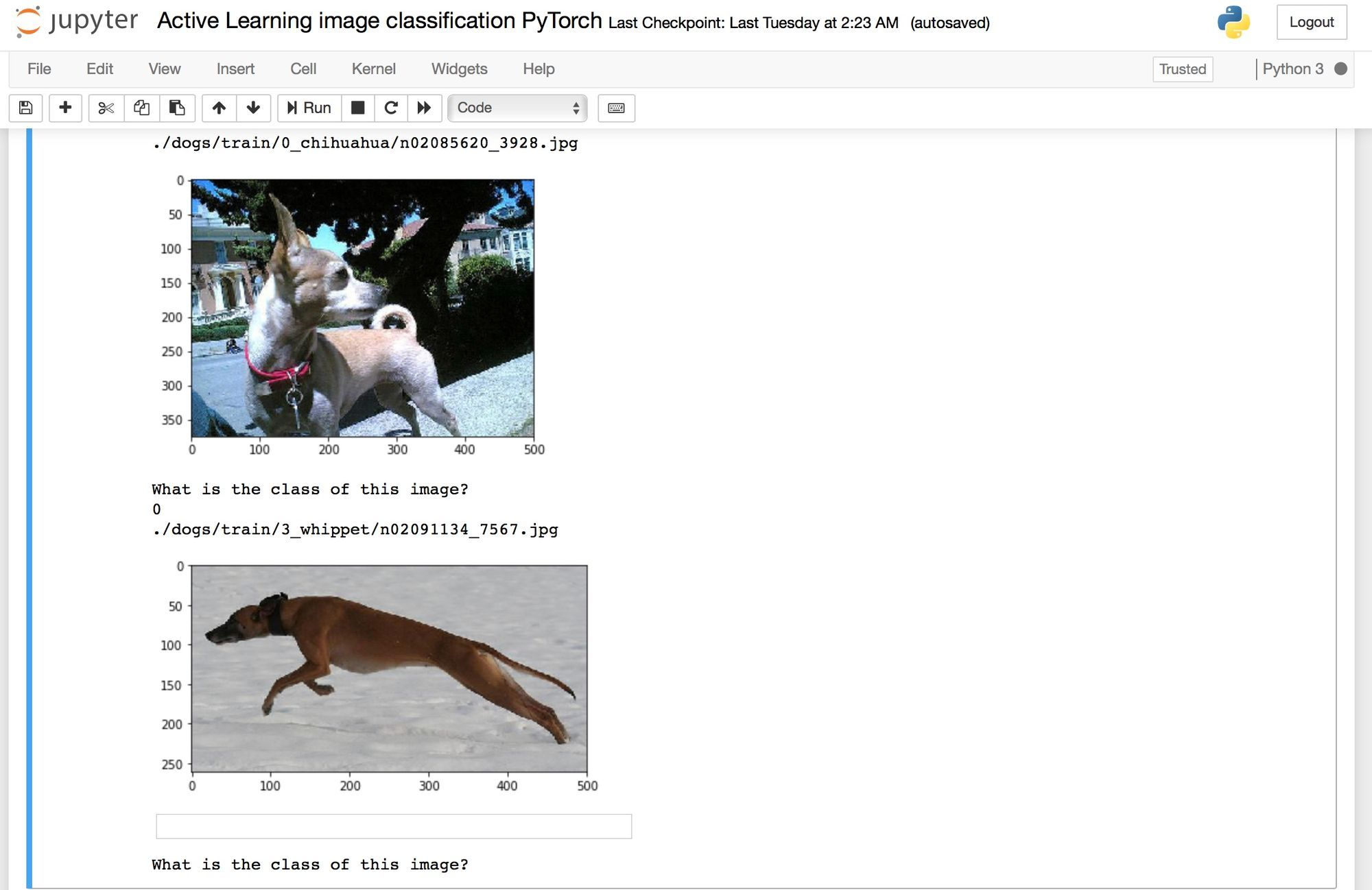
You are presented with query_size dog images to label, one at a time.

Much to my disappointment, the margin query strategy did not focus solely on the minituare vs. standard sized poodles. On the other hand, once a chihuahua and a whippet get resized to 224x224, can we really blame the neural network for having trouble distinguishing the two?

Results: is Active Learning worth it?

What we did above looks considerably more involved than training a good old supervised classifier. When might it be worth the trouble? Mainly when labeling the data is expensive, or otherwise difficult. Even with the toy example used here, we can see the benefits of employing a non-trivial (meaning, non-random) query strategy. Consider this plot of the test accuracy vs. number of labeled training samples:

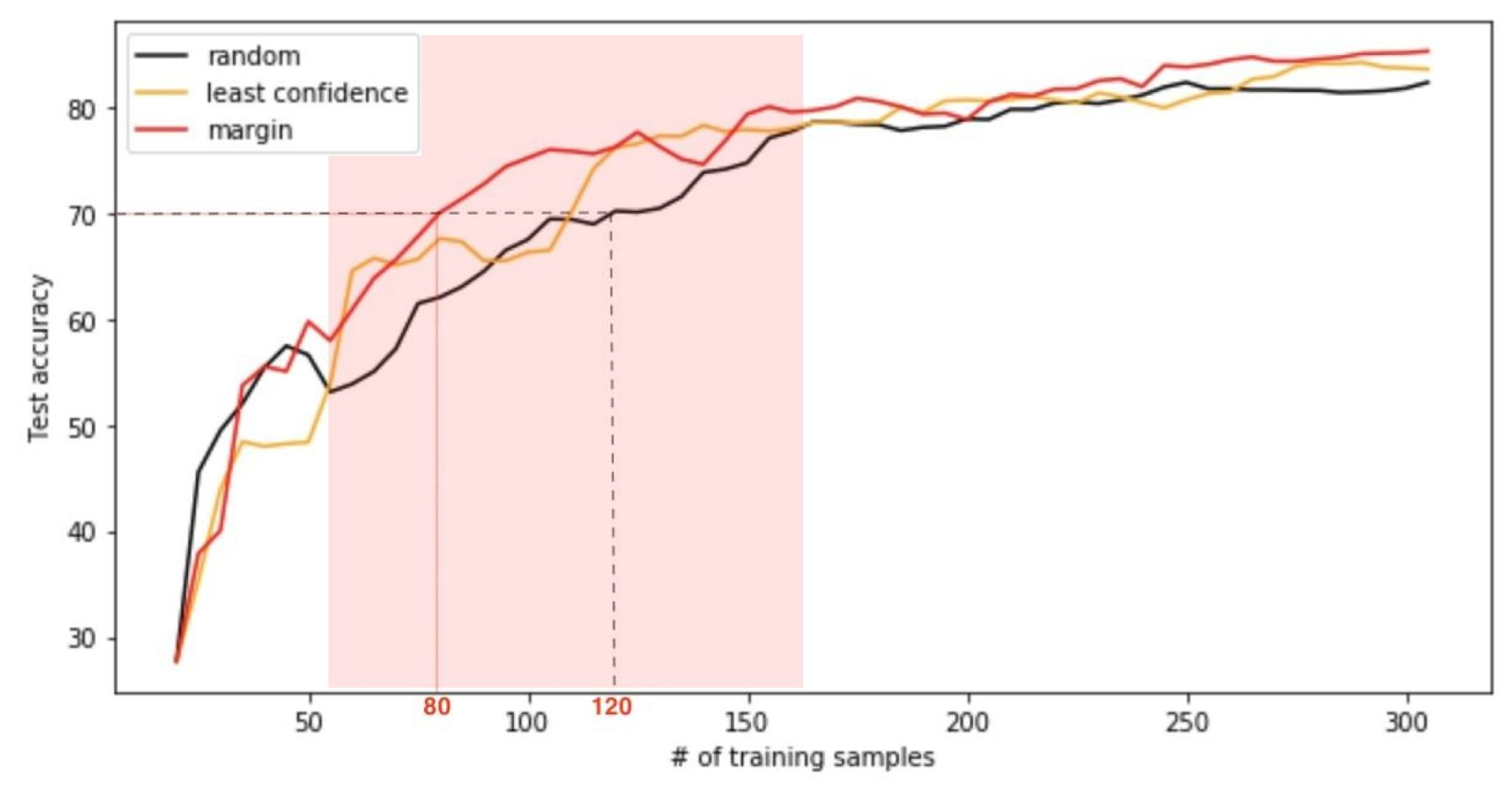
Here we start with merely 20 labeled images, so, even pre-trained, our classifier is understandably unhelpful in determining which samples would be most informative when labeled. (This can be seen from the black curve going above the orange and red ones in the first stage of the training - to the left of the red shaded area.) Once enough training samples have been labeled, however, active learning starts to shine. In the intermediate regime (shown in red), if we compare how much more data it takes random sampling to reach the accuracy achieved by the margin query strategy we'll mostly be in the 30%-50% range. Once a larger quantity of data is labeled, the three query strategies show similar performance once again (region on the right). Thus, depending on the nature of our problem and the level of performance that we wish to obtain, we can potentially reduce the data labeling costs by up to 50% through active learning! Granted, these savings come at an extra cost in compute time. Yet, with GPU computing becoming increasingly more affordable, the future of active learning is looking bright 😎